|
||
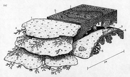
| Drawings of Permian reefs. (Wood, 1998) |
EARLY TRIASSIC AFTERMATH, SECTION 1
In addition to the major extinction, however, there is an aspect of the end-Permian catastrophe which makes it quite unique. The transition from the Permian to the Triassic was not merely a transition from one geological period to another, it also marked the passing of the Paleozoic Era and the start of the Mesozoic. It was as if the transition represented not just the coming of a new year, but a whole new millennium.
The Paleozoic had lasted from about 543
million years ago until about 250 million years ago, a period
of almost 300 million years, and more than half of the eon of
visible life, the Phanerozoic. When recovery from the Permian
extinction did occur, the new compliment of organisms was substantially
different from the old. What is commonly known as the Age of Trilobites
had passed, and the Age of Dinosaurs -- though without any dinosaurs
in its earliest stages -- had arrived. (See APPENDIX
2: A GALLERY OF PERMIAN-TRIASSIC CREATURES for pictures of
both older and newer organisms.)
But it was
not only that the recovery ushered in a dramatically different
biota from that which had gone before. The recovery after the
end of the Permian was delayed for millions, perhaps tens of millions
of years. The Permian extinction event had left a depleted planet,
one where the survivors had to face challenges for which the evolutionary
process had not prepared them. Many of the organisms with which
they had shared the Earth were gone: the plants the herbivores
consumed, prey and predators, disease organisms as well as helpful
symbionts. The entire biosphere required readjustment and reorganization.
During the millions of years which followed the end of the Permian,
the survivors struggled with exceptionally harsh and unfamiliar
conditions. The immediate post-Permian world, however, does provide
insight into the nature of the catastrophe itself.
The Reef Gap
Today we think of reefs essentially as coral reefs. A coral reef is, obviously, a reef made out of coral, which is the skeleton produced by a particular group of marine organisms. These organisms are anthozoans, part of a large and important subdivision (phylum) of the animals called cnidarians (pronounced ny-DARE-ee-ans). The better-known cnidarians include jellyfish and sea anemones.
The coral-building anthozoans themselves are minute organisms which use stinging cells to kill other tiny marine organisms that provide part of their subsistence. Many also possess photosynthetic algae (photosymbionts, referred to by coral specialists as "zooxanthellae") in their tissues (making them what is known as hermatypic corals), which provide the major source of food.
Coral-building anthozoans live together
as colonies that construct elaborate skeletons made of calcium
carbonate (CaCO¸3). The numerous skeletons of many different
kinds of anthozoans living in the same area constitute coral reefs.
These reefs provide food and shelter, including breeding grounds,
for many other marine creatures, like mollusks, crustaceans, and
fish. Consequently, while today's coral reefs comprise only a
small portion of the total marine environment, they harbor about
a quarter of all marine species. Earlier in Earth's history, reefs
provided similar shelter, food, and nurseries for marine species.
Permian Reefs and Reef Organisms
But the reefs of the Permian were not primarily coral reefs. Although reefs have existed throughout much of the history of life, they have been constructed by many different kinds of organisms. The same conditions that have attracted today's coral anthozoans to build reefs -- relatively warm, shallow (needed for sunlight for photosynthesis!) coastal marine settings -- have in the past attracted numerous other organisms to stake their own claims in these hospitable surroundings.
Permian reefs were not the elaborate and often towering (some are almost half a kilometer -- a quarter of a mile or so -- in height) constructs that today follow tropical coastlines and ring Pacific islands. Indeed, many paleontologists (for example, Flügel, 1994) prefer to label Permian reefs as mud mounds (built up from carbonate sludge) and/or reef mounds, which incorporated larger, skeleton-building organisms. But there were at least some highly developed reefs with a biotic diversity and a structural complexity approaching those of modern reefs. These fossil reefs display a reef zonation with fore-reef talus (debris shed from the reef face), a reef slope, crest, flat, and back-reef lagoon, though not the strong, surf resistant outer frameworks found in contemporary reefs (Wood, 1998). An outstanding example of such a reef, from the Late Permian, is the Capitan Reef of southwestern Texas and southeastern New Mexico (Wood, 1998; Scholle, 1999)..
The Permian reefs did include coral building organisms, but these anthozoans were different from those of today (called scleractinians or hexacorals). Permian corals were either rugose corals or tabulate corals, both of which had evolved in the early Paleozoic, and -- with some setbacks along the way -- had survived to the end of the Permian, when both groups were wiped out (though tabulates may have gone before the end; Boardman, 1987).
Permian reefs were mainly constructed by organisms referred to as problematica, calcareous algae, bryozoans, echinoderms, and calcareous sponges. Problematica (or, in this case, microproblematica because of their small size) are enigmatic organisms which are hard to classify because they do not seem to have left any clear descendants (or even close relatives) whose activities and remains might provide clues to their ancestors' identity. These enigmatic organisms are therefore known to paleontologists as problematica (problematicum is the singular form) for their problematic relation to other living things. (Generally speaking, the farther back in time we look, the more problematica there are, because many extinct organisms have no clear descendants. Nonetheless, paleontologists do make educated guesses.)
|
||
| Drawings of Permian reefs. (Wood, 1998) |
Among the Permian major reef-building
organisms are the problematicum Archaeolithoporella, a
possible calcareous red alga (a rhodophyte; Mazzullo and Cys,
1977) or, perhaps, more likely, a calcifying microbe (Grotzinger
and Knoll, 1995) that deposited carbonate crusts on other reef
organisms and carbonate mud accumulations. These crusts comprise
numerous thin layers; it has been suggested that they may have
grown in dim cavities within the reefs.
Archaeolithoporella, a Permian reef builder. At Capitan
Reef, in Guadalupe Mountains National Park, Texas. (Photo by Scholle,
1999)

Another Permian reef problematicum is Tubiphytes, a group whose members formed crusts as well as helping build reef structures. Tubiphytes may also be a calcareous alga, or an unusual kind of foraminifer. Calcareous algae are seaweeds, eukaryotes (organisms with complex cells) that produce calcium carbonate (hence "calcareous") skeletons, probably in order to discourage grazing by other organisms. Their calcium carbonate skeletons contribute to the structure of reefs. Despite our inability to satisfactorily classify these organisms, they were undeniably important parts of Permian reef communities (Flügel, 1994).
Bryozoans are animals, of which they constitute a major subdivision (phylum). They are tiny marine organisms which live in colonies and produce typically small (though some may reach a meter in size) but intricate -- sometimes branching, columnar, spiral, lacy, or platy, sometimes encrusting -- skeletons. There are plenty of bryozoans around today, but most of them are different from those that were common in the Permian.
Echinoderms (today's starfish and sea urchins) are another animal phylum. Paleozoic echinoderms included not merely starfish (asteroids: but not to be confused with the big rocks that wander through the solar system!) and sea urchins (echinoids), but also numerous echinoderms which attached themselves by stalks to the sea floor, and possessed tentacles that resembled petals. These echinoderms, called crinoids, are therefore also referred to as sea lilies, and are often found in limestone quarries in the American Midwest. Echinoderms build their skeletons of small plates of calcium carbonate (called ossicles). When echinoderms die, the ossicles separate, contributing lots of small bits of skeleton to the reef debris.
Sponges were also significant members of the Permian reef community. These are real sponges, not the cellulose versions that we buy for kitchen use, nor the luffas (or loofahs) that are used in the bath (which are actually made of vegetable fibers from dried gourds). Occasionally one sees the fibrous skeletons of real sponges being sold in auto supply stores: they are irregular, have holes of varied sizes, and are naturally a dirty yellow color. (In their marine environments, live sponges display a wide variety of colors: white, yellow, orange, red, purple, blue, green, brown. Some are even bioluminescent: Margulis and Schwartz, 1982.) These are the skeletons of sponges which are made of organic material (spongin).
Sponges are multicellular marine animals that are typically attached to the seafloor by root-like structures called holdfasts. They pump water through their bodies, filtering out the small organic particles they consume for food. Whether sponges are truly animals (metazoans) has been the subject of an ongoing debate among those who study them. Because of their simple organization and the relative primitiveness of their cells, sponges are quite different from other animals. Moreover, because of their simple organization, they did not give rise to more complex organisms. But despite their unique attributes, the consensus seems now to be that they are properly classified (as a phylum) among the animals.
Most sponges have skeletons. In addition
to those constructed from organic fibers, there are also sponges
which build skeletons from silica (glass; these sponges are referred
to as glass sponges, or, technically, hyalosponges) and calcium
carbonate (calcareous sponges, or, for short, calcisponges). In
addition to the skeletons, sponges often contain large numbers
of tiny, needle-like spines called spicules. These spicules probably
serve a defensive purpose, discouraging predatory organisms from
grazing on the otherwise vulnerable animals. Of the sponges, it
is the calcisponges -- and, in particular, large, plate-like sponges
-- which most helped build the Permian reefs.
In addition to these reef-building organisms, other groups (phyla) also made their own shell and skeletal contributions to the Permian reefs:
Foraminifera (forams) are mostly tiny marine organisms, though some may grow up to a few centimeters (about an inch) in diameter. Forams are a major subdivision (phylum) of the kingdom Protoctista, a large group of single-celled eukaryotes. They possess porous shells called tests, usually composed of organics and calcium carbonate, although some employ silica (silicon dioxide, equivalent to glass) or agglutinate (glue together) their tests from bits of sand. One notable group of Paleozoic forams, the fusulinids, were about the size of rice grains (but with some members reaching 1.4 cm -- half an inch), and possibly had photosynthetic symbionts. The fusulinids were plentiful up until the end of the Permian, when they too went extinct.
Mollusks include many forms of large shelled organisms like today's snails (gastropods), clams, mussels, and oysters (bivalves), slugs, and, perhaps surprisingly, squid, octopi, and the chambered nautilus (cephalopods). The mollusks of the Permian were not the same as those of today, of course, but there did exist a wide range of gastropods, bivalves, and the ammonites, a group of large cephalopods which superficially resemble the chambered nautilus of today's south Pacific but are actually quite different. Freely moving in the ocean's waters, the ammonites would not have contributed to the making of Permian reefs, but the shells of bivalves and snails would have added to the buildup of calcium carbonate debris.
Brachiopods (often referred to as lamp-shells, for the oil lamps of the classical Greek and Roman eras), were then a major group of bivalves that today is almost extinct. Brachiopods superficially resemble bivalve mollusks but are totally different -- so different, in fact, that they each are placed in different major subdivisions (phyla) of the animals. Both groups make their livings by filtering food particles from seawater, though they employ quite distinct feeding mechanisms to do so.
The mass of Permian reefs was held together
in part with accumulations of brown-colored carbonate ooze, called
micrite, and carbonate cements, which often crystallized in a
grape-cluster (botryoidal) aggregates. The Permian "mud mounds"
consisted primarily of micrite sludge.
In the Late Permian, these reefs were thriving. And then they were gone. In a geologic eyeblink, the reefs of the Permian disappeared. And they were not replaced, not immediately, that is. The reefs became fossil monoliths, and many of the organisms which had created them -- rugose corals, fusulinids, and many echinoderms, bryozoans, and brachiopods -- disappeared forever. For ten million years, throughout the Early Triassic, there were no reefs. Only a few carbonate buildups, some perhaps from lagoons rather than from along seacoasts, have been discovered, and the dates of these are often uncertain. Where present, they are composed of calcareous algae and lack larger organisms. To paleontologists, this period is known as the Early Triassic Reef Gap.
It was only during the Middle Triassic that reefs began to come back. Although these reefs were still considered by some scientists to be mere mud mounds and reef mounds, their constituents had changed. Apparently, none of the major Permian reef builders survived the events at the end of that period (Flügel, 1994).
Obviously, significant evolutionary changes could have taken place among reef-building organisms during the ten million years that followed the Permian extinction, and some of the organisms that emerged in the Middle Triassic could have been descendants or close relatives of those that disappeared at the Permian's end. But there seems to be little question that the reef-builders of the Middle Triassic were different. Even when the Triassic organisms appear similar, the poor preservation of some reef-builders or their vastly differing ecological settings makes the possibility that some are identical to Permian reef organisms quite unlikely.
While calcisponges were again present
in reefs of the Middle Triassic, these calcisponges were not the
same as those of the Permian. Algae and microproblematica were
also different. The microproblematicum Tubiphytes of the Middle
Triassic exhibit distinct differences from that of the Permian,
for example (Flügel, 1994). Archaeolithoporella, a dominant
reef-builder of the Permian, was gone forever.
The Coal Gap
Coal is derived from peat, and peat itself forms in mires: freshwater environments (bogs, moors, swamps, and other wetlands) where the lack of oxygen inhibits, then prohibits, decay. Bits of plant material accumulating in such environments eventually are transformed into a kind of organic slurry, and larger pieces of wood and other plant material become waterlogged and thereby preserved. In the process, called humification, cellulose leaves behind a carbon-enriched residue and releases water and the gases carbon dioxide and methane.
2(C¸6H¸10O¸5) Æ
C¸8H¸10O¸5 +
2CO¸2 +
2CH¸4 + H¸2O
cellulose (yields)
humified residue + carbon dioxide + methane + water
The methane -- often appropriately referred to in this setting as swamp gas or marsh gas -- occasionally catches fire, and faint blue "will-o-the wisp" flames play across the surface of still waters (Duff, 1993).
Peatlands are extensive throughout the globe, in colder environments where peat develops in the shallow depressions left by former glaciers, in tropical regions, and even in such temperate and subtropical areas as Delaware's Great Dismal Swamp and Florida's Everglades and Ofekenokee Swamp. As they are compacted by the further accumulation of plant material, the deeper layers of peat are increasingly squeezed of their water. Deeper burial, under influxes of sediment, together with the heat that comes with depth, further drives off the water and other volatiles. Eventually the peat is converted first into lignite, a brown coal, and then into the more familiar forms of black coal: bituminous or soft coal, and anthracite or hard coal. The process, of course, is a slow one, taking millions to tens of millions of years (Duff, 1993).
Coal has probably been forming ever since plants took to the land, which occurred in about the middle of the Silurian Period (roughly 425 million years ago). By the end of the Devonian (about 360 million years ago), there were full forests -- and the first geologic appearance of coal. This coal was mainly produced in tropical and subtropical regions (subtropical regions are like today's Florida). During the next geologic period, there was extensive coal formation, in regions from the tropics to the cooler parts of the temperate zone, at almost 60° from the Equator. So much coal was produced that its plenitude provided the name for the period: the Carboniferous -- literally, the carbon (here, coal) making.
In the Permian the main regions where
coal was being produced were in the temperate zone; major coal
formation had shifted from the tropics. The Permian world left
extensive deposits of coal, found today in China, India, Australia,
Africa, and Antarctica.
Red Beds
And then, as with the reefs, peat and coal formation ceased for the ten million years of the Early Triassic. When it did resume, during the Middle Triassic, the coal seams were rare and thin. This period is known as the coal gap (Veevers, 1994; Retallack, 1996). What is particularly striking is that the areas that had previously been sites of coal formation were replaced by red beds. Red beds are sedimentary strata (hence, beds) colored red by the presence of hematite, ferric oxide (Fe¸2O¸3). The sedimentary strata are composed of sandstone, siltstone (smaller sized particles), and shale, sometimes with interbeds of conglomerate, marl, or limestone.
Red beds are generally taken to be indicators of arid conditions, often inundated by seasonal -- monsoonal rains. They derive their red coloring from thin coatings of hematite (rust) on their constituent grains. Many scientists believe that these hematite veneers are the result of highly oxidizing conditions that may have attended the deposition and weathering of the red beds. (But this idea has recently been challenged, because not all rocks formed in desert conditions are red, and because some red beds have clearly formed mild, humid, and temperate climates; see Sheldon, 2002. It seems likely, however, that many red beds were indeed formed in arid conditions.)
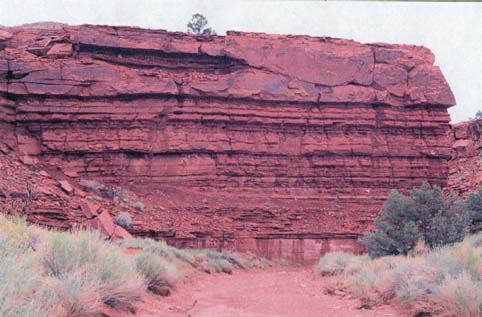
Red beds are common throughout the US Southwest, where arid conditions prevent soil formation and vegetative cover, and allow rock outcrops to be exposed. Much of the "Canyon Country" of the Four Corners (Utah, Colorado, New Mexico and Arizona) area displays these beds. Red beds are not exclusively from the Early Triassic, however. The red beds of the American Southwest include Permian, Triassic, and Jurassic formations. Only the red beds of the Moenkopi Formation, visible in Zion National Park, at Capitol Reef in central Utah, and elsewhere in the Southwest, represent those Early Triassic red beds that throughout much of the world followed the end of Permian coal formation.
It is not the presence of red beds which is striking about the Early Triassic -- after all, red beds are commonly found in sedimentary strata -- but rather that they abruptly followed the deposition of coal in many areas where coal was being formed right at the end of the Permian. It was only in the Late Triassic that coal formation again reached Permian levels.
In attempting to discover why peat and coal production ceased completely during the Early Triassic, and resumed only slightly in the Middle Triassic, paleobotanist Greg Retallack and fellow scientists (1996) examined several proposals. The proposal that mires might have been overwhelmed by an influx of acid from Siberian Traps aerosol sulfates (McCartney, 1990) was rejected because any acid rain that might have been produced would only have had short-term -- not ten million year -- consequences. The possibility that hot and arid climate conditions could have stifled peat production (Worsley, 1994) was rejected because there were still temperate conditions in much of the Triassic world. Similarly, the suggestion that decomposers like fungi or that insect or vertebrate consumers of peat may have become more effective (Moore and Worsley, 1994) was dismissed because the end-Permian extinctions had reduced their diversity (Retallack, 1996).
After examining these and other proposals
for the cessation of peat and coal formation, Retallack and his
fellow investigators conclude that the coal gap must have been
due to the extinction of peat-forming plants in the end-Permian
extinction. They note that relatively few plants are adapted to
the harsh conditions -- those of waterlogged, acidic, dysaerobic
environments -- in which peat is formed. The extinctions of the
end-Permian decimated these plants, and, Retallack and his associates
believe, it took many millions of years for other plants to become
tolerant of such conditions (Retallack, 1996).
The Chert Gap
What is perhaps most surprising about the Early Triassic Chert Gap is that it came after a major and probably worldwide episode of exceptional chert deposition, the 30 million year long Permian Chert Event (Murchey and Jones, 1992; Beauchamp and Baud, 2002). Chert is predominantly composed of silicon dioxide (also called silica; SiO¸2), the same stuff as glass. Many marine organisms construct their skeletons of silica, which is dissolved in seawater.
Prominent among these organisms are the radiolarians, single-celled eukaryotes (protoctists) which filter or actively prey upon other organisms for food. Some obtain food from symbiotic photosynthetic algae (zooxanthellae). Radiolarians construct tiny, lacy skeletons of opal, another form of silica. When radiolarians die, these skeletons drop to the ocean floor, where they may accumulate in enormous numbers. Together they constitute what is called radiolarian ooze. As with all sediments, this ooze eventually becomes compacted and hardened by the weight of further accumulations above, becoming chert.
On occasion, this chert is pushed up onto the continents, as it has been in the Marin Headlands. There the folds of great red chert beds define the topography. These cherts are called ribbon cherts for obvious reasons. They were deposited in deep water some 200 to 100 million years ago, and were scraped off the ocean floor as the former Farallon Plate, an oceanic plate, subducted beneath the North American continent. The Marin Headlands' radiolarian chert is up to about 80 meters (yards) thick, and comprises part of the coastal geological formations known as the Franciscan Complex.
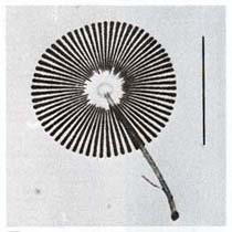
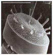
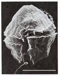
Because many creatures construct their skeletons from silica, chert may be produced in several ways. The chert of the Permian Chert Event was produced primarily by radiolarians and glass sponges (hyalosponges: hyalo is Greek for glass). The hyalosponges possess both sharp glass spicules (needles), and, in some species, glass skeletons. Perhaps the most famous example of a glass sponge is today's Venus flower basket (Euplectella), which produces an intricate, fragile, and beautiful skeleton (see below). When radiolarians and sponges with glass spicules and skeletons die, the glass becomes part of the seafloor debris.
In the middle of the Early Permian (roughly 275 million years ago), biogenic silica began to be deposited along the northwest margin of Pangea (the area that now stretches from Nevada and across the Canadian Arctic, although much of today's North American West Coast -- California, Oregon, Washington, British Columbia, Alaska -- was not yet part of the continent). These early deposits were not preserved as chert, but rather as cherty carbonates and mudrocks (Beauchamp and Baud, 2002). Later in the Early Permian, massive chert deposition began in deep water far distant from the Pangean coast. Closer to shore, in shallower waters, changes in carbonate sedimentation reflected a cooling of this part of the ocean.
The Early Permian chert deposits mark the onset of the Permian Chert Event. These deposits are primarily composed of sponge spicules, and are referred to as spiculitic chert. The hyalosponges were so successful in the colder waters of Panthalassa that they are labeled "silica factories." As the Permian progressed, these silica factories moved ever closer to the coast, gradually displacing the more cold-adapted carbonate-secreting organisms of the shallow water environments, just as the cold water carbonates had previously replaced the warm water carbonates earlier in the Permian. By the Late Permian, chert accumulation in what is now the Canadian Arctic reached a kilometer (6/10ths of a mile) thick, and chert-rich strata were being created worldwide, even along the margins of the Tethys (Beauchamp and Baud, 2002).
Off northwest Pangea, ocean temperatures cooled over the 30 million year period prior to the end of the Permian. Because all of Pangea moved north during that time, that oceanic cooling presumably derived in large part from the seasonal melting of sea ice. Cold water currents in this region (then the northwest of Pangea, today West Coast of North America) are to be expected, because ordinary ocean circulation carries subarctic water south along the coast.
But the extent of the cold was unusual: "It led to oceanic conditions much colder than normally expected from [those] palaeolatitudes, and the influence of cold northern water was felt as far south as southern Nevada" (Beauchamp and Baud, 2002). At the time, this part of the world was no further north than tropical Central America is today (about 15°N). What is now the Canadian Arctic lay at about 35°N, approximately the latitude of today's Los Angeles. This part of Panthalassa, therefore, was exceptionally cold.
During this same time, Earth was emerging from the 80 million-year-long Late Paleozoic ice age, which seems to have ended only some five million years before the end of the Permian, though some scientists (as, Veevers, 1994) believe it may have lasted to the end of the Permian itself. (This ice age, now referred to as the Late Paleozoic Gondwanan Ice Age [LPGIA], may actually be comprised of a series of "short-duration" glacial episodes, each lasting no more than about five million years, together spanning from 320 million years ago to 265 million years ago, or only 55 million years in total: Fielding, 2006.) By about five million years before the boundary, however, the great continental ice sheets had melted. Nonetheless, it does seem possible that cold climatic conditions could have persisted to the end of the Permian, or that a new episode of frigid global climate was beginning.
Surprisingly, the Permian Chert Event
also may have ended before the Permian-Triassic boundary -- not
by much, but by some. Originally it was thought that the termination
of the Chert Event came exactly at the boundary, but more recent
observations have challenged that determination. It now appears
that the end of the Chert Event may lie, at least in one geological
setting (the Sverdrup Basin, now a part of the Canadian Arctic),
some 32 meters (about 100 feet) below the actual Permian-Triassic
boundary (Beauchamp and Baud, 2002).
Using the index fossil that first appears at the exact beginning of the Triassic (the conodont -- a marine worm whose tiny jaw bones are well preserved -- Hindeodus parvus), the Permian-Triassic boundary can be unambiguously determined in certain rocks of the Canadian Arctic's Sverdrup Basin. This area, which was an oceanic basin in the late Paleozoic and early Mesozoic, now reveals itself as the north of Melville Island, the west of Ellesmere Island, and Axel Heiberg and all of the other Canadian Arctic islands in between, provides a look at the rocks of the Permian Chert Event.
But these same rocks indicate that chert formation ceased 32 meters below the Permian-Triassic boundary. The amount of time that passed between the end of chert deposition and the P-T boundary depends on the rate of sedimentation, which cannot be determined precisely. But a not unreasonable guess would be that the 32 meters of sediment represent a time interval from tens of thousands to possibly a million years.
This presents an enigma, because one's natural expectation is that chert deposition should have been just another of the many things which were impacted by the end-Permian catastrophe. But perhaps not. Perhaps, for some reason, chert deposition did indeed cease several tens of thousands to a million years before the Permian-Triassic boundary as marked.
As a former arm of the sea in which this rock section resides, the Sverdrup Basin could have become closed off from the open ocean (such things do occur, not infrequently). Or an early, minor eruption of the Siberian Traps could have showered enough ash over the area that the filters of the filter-feeding radiolarians and sponges became clogged, killing them off. Other volcanic effects, like acid rain or toxic gas could also have taken their toll.
Or, as sometimes does happen (and did once already in this area, when the P-T boundary was thought to be lower down and coincident with the end of the Chert Event), perhaps the boundary marker is in the wrong place. Perhaps the fossil conodont Hindeodus parvus does not correctly delineate the Permian-Triassic boundary. Or perhaps it does so elsewhere, but does not in this particular area.
Clearly the scientists Beauchamp and Baud are suspicious about whether Hindeodus parvus accurately defines the boundary. They write, "...the demise of the silica factories, not only in the Sverdrup Basin, but around the world is referred to as an 'end-Permian' event or a 'latest Permian' event. The same applies to a number of other biological, geochemical and environmental events that accompanied the transition from the Palaeozoic to the Mesozoic. These events invariably occurred prior to the first appearance of H. parvus" (Beauchamp and Baud, 2002). This dispute with the use of H. parvus as the boundary marker finds support with others, who note that the fossil first appears above the boundary placement determined by fossil pollen (Twitchett, 2001; Wignall and Twitchett, 2002). Even at Meishan, China, where the official geological marker for the Permian-Triassic boundary has been placed, "the mass extinction and sharp negative excursion in d^13C [that is, the sharp negative excursion in carbon isotopes, presumably indicative of massive methane release] are slightly older than the formal stratigraphic boundary" (Ward, 2005; see also Xie, 2005).
On the other hand, it may be that what has been determined to be the boundary does not accurately reflect the time of the catastrophe at the end of the Permian. In South China, the start of the extinction event -- placed by radiometric dating at 251.4 million years ago -- falls well before the boundary, at about 250.8 million years ago (Jin, 2000). This sort of discrepancy, almost unavoidable considering the slight uncertainties in radiometric dating (from 0.1% to 1%) and the differences among the personnel, techniques, and equipment of the world's few geochronology centers, has prompted a call for increased accuracy in such measurements (Kerr, 2003. A call for telling better time over the eons).
Further examination of the area may provide additional evidence. Or it may not: when scientists reach back through millions of years of time (or, in this case, a quarter of a billion), it is inevitable that there should be mysteries which have no answers. Why, for example, did all the dinosaurs and major marine reptiles die off at the end of the Cretaceous, but not the crocodiles? (That's one which continues to perplex my paleontologist friend and former professor, Richard Cowen.) Simply, we may not ever know.
But we do know that following the Permian Chert Event there was an Early Triassic Chert Gap, which is first noted in one area of the Sverdrup Basin as being marked by "finely-laminated, pyrite-rich siltstone" (Beauchamp and Baud, 2002). There are thin (1-2 cm; about a half to almost a full inch) beds of mud carbonate (micrite) that contain the "ghosts" of dissolved sponge spicules. Chert deposition, or at least its preservation, had ceased.
To geologists, this rock outcrop provides a wealth of information. Conditions in the far north of Panthalassa had changed sufficiently that the glass sponge spicules were being dissolved rather than preserved, likely the consequence of a warmer ocean. The pyrite is a clear indication that the region's water had turned anoxic, because pyrite (iron sulfide) is produced only where oxygen is not present. Probably most important, the fine laminations of the siltstone -- silt itself being comprised of fine grains -- shows that these ocean sediments were not disturbed by bioturbation.
Bioturbation is the geologist's term for the churning of sediment by aquatic organisms (it occurs in both marine and freshwater settings) such as worms, crustaceans, and mollusks, which displace sediment as they burrow through it in search of shelter or food. (Today large creatures like walruses also bioturbate as they rake the sediment with their tusks for the mollusks that lie within.) The finely-laminated siltstone -- with its lack of bioturbation -- is an unequivocal sign that organisms which used to live there disappeared, victims of the great biological catastrophe at the end of the Permian.
Glass sponges, however, were not the only marine organisms with silica skeletons that were decimated. So also were radiolarians, single-celled creatures that consume phytoplankton (Racki, 1999; Racki and Cordey, 2000). Radiolarians, whose radial spines give them their name, are eukaryotic plankton (floating organisms) which flourish in warm waters. The floors of equatorial oceans frequently are covered with radiolarian ooze, composed of the skeletons of countless numbers of these creatures. Eventually the accumulated ooze can solidify into chert. While Early Triassic oceanic anoxia likely drove most hyalosponges to extinction, and caused the cessation of hyalosponge chert production, it seems that the lack of radiolarian chert was due not only to the die-off of the radiolarians themselves, but also to the warmer marine conditions in the deep equatorial ocean, which would have enhanced silica dissolution.
The Early Triassic Chert Gap lasted for
some eight to ten million years. (For the radiolarians, the gap
may have been as long as 13 million years: Racki, 1999.) In what
is now the Canadian Arctic, this period is characterized by rare
fossils, significant influx of sediment, and, in adjacent terrestrial
environments, red beds and other indicators of arid conditions.
No chert is present, even as small nodules. Indeed, there is nowhere
on the planet which displays chert from the earliest part of the
Triassic. It was only later in the Early Triassic that limited
silica deposition resumed, and later still before genuine chert
beds reappeared, at about the beginning of the Middle Triassic.
The Early Triassic also presents evidence of other unusual conditions. The conifers which had constituted a major component of the central Laurasian (what is now the Europe) forests had been hard hit at the end of the Permian, and did not recover until the Middle Triassic (Looy, 1999). The presence in Triassic soils of the unusual green crystalline mineral berthierine seems to indicate low atmospheric oxygen, perhaps partly drawn down by atmospheric methane (Sheldon and Retallack, 2002; but see also Huggett and Hesselbo, 2003, and the reply of Sheldon and Retallack, 2003), but also likely the consequence of the impairment of photosynthesizers.
Despite the lack of evidence regarding what happened to phytoplankton without fossilizable hard parts, it is clear that ecological conditions on the planet, and more specifically in the ocean, were greatly disturbed. Following the initial negative carbon isotope excursion at the Permian-Triassic boundary, the carbon cycle continued to reflect serious perturbations for the next 4 to 8 million years, into the early part of the Middle Triassic. A second negative carbon isotope shift was recorded a million or so years after the boundary, followed by a major, long-term positive shift, then a third negative shift that may have been even greater than that of the boundary section, a brief return to relative normalcy, and another negative and positive excursion, all within the 4 to 8 million year interval beginning with the extinction and ending in the early Middle Triassic (Payne, 2004).
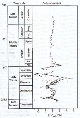
Aside from confirming that the Early Triassic was a period of continual major instability, the findings provide no insight into the possible causes of the disturbances. As the discoverers of the carbon fluctuations note, the fluctuations could either themselves represent repeated environmental disturbances, or the consequences of those disturbances, as ecosystems were decimated and rebuilt (Payne, 2004). In other words, the carbon isotope changes could be telling us either of causes (for example, methane outbursts) or consequences (for example, severe disturbances of the biosphere).
In the marine realm, there may be at least a partial explanation for the fluctuations. Because the ocean is normally a quite stable environment in terms of chemistry and temperature, many marine organisms thrive in narrowly defined but stable living conditions. Where there is normally little environmental change, organisms adapted to those conditions fare well. But in such situations, small ecological variations can have significant effects. The slight warming of the eastern North Atlantic over the past 40 years, for example, has resulted in the movement of warm-water phytoplankton some 1000 kilometers (600 miles) further to the north (Beaugrand, 2002).
There is, however, evidence of far greater changes in marine phytoplankton at the Permian-Triassic transition. With millions of years of altered conditions in the oceans, it should not be surprising that there were enormous changes in oceanic organisms. During the Paleozoic, the dominant marine eukaryotic phytoplankton were the green algae (chlorophytes). (Almost all land plants evolved from green algae.) These organisms possess chloroplasts (the organelles -- "little organs" -- that conduct photosynthesis) with specific types of chlorophyll (the pigment that facilitates photosynthesis). Together, these organisms are referred to as the green plastid lineage (Falkowski, 2004).
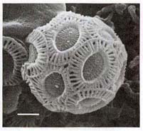
Today, by contrast, the dominant marine eukaryotic phytoplankton belong to the red plastid lineage. This lineage derives from red algae (rhodophytes), and possess their own types of chlorophyll. Among the members of this lineage are single-celled organisms called dinoflagellates (most are of the red plastid lineage, though a few are of the green plastid lineage), coccolithophorids, and diatoms (Falkowski, 2004). These creatures are among the major photosynthesizers of the modern ocean, and, as such, contribute large amounts of oxygen to the atmosphere.
Dinoflagellates have bodies covered with cellulose plates. They are the organisms responsible for the toxic "red tides" which periodically cause the closing of beaches and engender prohibitions against the eating of certain fish and shellfish (which themselves have consumed dinoflagellates and are therefore also toxic). Some species are bioluminescent, and produce a fluorescent glow in breaking waves, particularly noticeable at dusk. Coccolithophorids have skeletons of calcium carbonate, and diatoms possess skeletons of silica. The remains of dinoflagellates are first found in the later Triassic; the skeletons of coccolithophorids also appear in the late Triassic; molecular evidence indicates that diatoms may have originated about the time of the Permian-Triassic boundary, though their skeletons are only found much later.
|
||||
|
|
All of these lines of evidence suggest that these red plastid lineage organisms may have been beneficiaries of the changed conditions of the Permian-Triassic transition. Presumably that transition began with the extinction of many of the organisms of the Permian oceans. Numerous other organisms probably were forced to live more marginal existences, and may not have survived the millions of years of the transition period. During that period, the remaining formerly dominant organisms struggled with organisms which previously themselves had been marginalized but which found new opportunities in the altered conditions, as well as with newly originated organisms more adapted to the new conditions.
In all likelihood, the biological constituents
of the oceans varied widely over the millennia as intense competition
among these creatures for light, nutrients, and living space characterized
the disordered world of the Late Permian and Early Triassic. During
this "warring [microbial] states" period, some microbial
assemblages presumably came into prominence, then, having exhausted
the nutrient supplies necessary for their existences, or having
flooded their environments with wastes toxic to their own continued
success, inevitably declined. (We often forget that the very success
of organisms can so alter their environments that they compromise
their own continued existence and actually create the conditions
in which other organisms can outcompete them.)
The intensity of that struggle and the major ecological swings
of the time are recorded in the wide swings of the carbon isotope
record (Payne, 2004), and in other geochemical and paleontological
evidence (for example, Xie, 2005). Other marine organisms are
likely to have been impacted by the ascendancy or decline of various
microbes: certainly the composition of the zooplankton, the planktonic
organisms which consume phytoplankton, would have shifted as their
foodstuffs changed. Organisms higher on the food chain would presumably
been affected as well.
In addition, increases in the numbers of dinoflagellates could
have resulted in greater "red tide" mortality, and population
increases in certain diatoms could have resulted in the disorientation
and deaths of vertebrates with highly complex nervous systems
by domoic acid poisoning. Although shellfish and fish are apparently
immune to such poisoning, organisms that consume them may not
be, as shown by the poisoning of many seabirds in the Monterey
Bay area of coastal California in the early 1990s, and the recent
demise of numerous sea lions. (Human beings also lack immunity,
and domoic acid concentrations in shellfish can produce what is
known as amnesiac shellfish poisoning, resulting in short-term
memory loss.) Even population changes among the humble cyanobacteria
could have taken their toll by means of their newly-discovered
nerve-damaging neurotoxins (Cox, 2005).
The ascent of the red plastid lineage to post-Paleozoic prominence has been traced to known characteristics of the Early Triassic oceans. The euxinic (high sulfide) marine conditions may have depleted the oceans of nitrate, an essential nutrient (Falkowski, 2004; see also Kuypers, 2005), conferring a competitive advantage on organisms (here including red plastids) which evolved a more complex system for obtaining their nutrients. The lower levels of oxygen may also have favored organisms (again, the red plastid lineage) which require more of certain trace metals (manganese, cobalt, cadmium) rather than others (zinc, copper) the supplies of which would have been reduced by the dysoxic conditions. Finally, the red plastid lineage organisms flourished in coastal environments, where oxygen supplies were greater than in the open ocean, which was preferred by members of the green plastid lineage (Falkowski, 2004).
If indeed the Permian phytoplankton (specifically the green plastid lineage) did suffer the extreme losses projected by this scenario -- and especially if the terrestrial oxygen producers suffered similar losses -- the extinction could have accomplished something the great methane release itself could not: a significant reduction of atmospheric oxygen. For despite the enormous amount of methane that was likely released, the quantity of oxygen in the atmosphere is vastly greater, and only a small part of that oxygen could have been directly drawn down through chemically combining with the methane. Cutting the supply of oxygen at its source, however, would have been devastating, and would have imposed a costly burden on all aerobic organisms. In view of the upheaval in the green and red plastid lineages, it does seem plausible that such a blow to the great free oxygen reservoir -- the air -- may have actually occurred.
There are several lines of evidence which
suggest that Late Permian and Early Triassic oxygen levels could
have been and probably were significantly affected by the ecological
changes of the time. Computer climate modeling (Schmittner, 2005)
of today's world indicates that the increase of freshwater (from
the melting of northern ice) rapidly results in a major reduction
in the normal North Atlantic oceanic circulation. This circulation
(referred to as the Atlantic meridional overturning circulation)
is responsible for pumping frigid, highly saline water (North
Atlantic Deep Water) down to the floor of the North Atlantic.
Without this input, according to the climate model, the North
Atlantic will quickly stratify, separating the nutrient-laden
waters of the deep ocean from the organisms that depend on them,
the phytoplankton of the surface ocean.
The phytoplankton, in other words, will face starvation conditions,
and will suffer population losses approaching 50%. Over time,
the circulation of both the Indian and Pacific Oceans will also
decline, and organisms there too will suffer significant losses
(Schmittner, 2005). Though the study's author does not examine
how atmospheric oxygen levels would be affected, the consequences
of a serious (roughly 50%) global phytoplankton decline are obvious:
about 1/6th to 1/4th of the global production of oxygen would
be cut off (phytoplankton account for about 1/3 [Campbell, 1987]
to 1/2 [Falkowski, 1998] of planet's oxygen production; the rest
being produced by terrestrial green plants). If phytoplankton
productivity were to continue at such low levels over geologically
extended periods, atmospheric oxygen levels would fall by at least
that amount.
In fact, a situation similar to that projected by the computer modeling has already begun to occur. Even the present mild warming (about 1°C; 1.8°F) of the northeastern Atlantic has resulted in an increase in phytoplankton abundance in colder, more northerly waters (as they warm), but a decrease in more southerly, warmer waters (presumably as they are denied deep water nutrients). Because these changes are happening to the organisms at the bottom of the food chain, all the other marine organisms (from zooplankton to fish, birds, and marine mammals) which depend upon the phytoplankton will also be affected (Edwards and Richardson, 2004; Richardson and Schoeman, 2004). Again, though the study does not specifically look at the oxygen production of the phytoplankton, this too will be affected.
The amount of oxygen in the atmosphere, however, depends on two basic factors, input and outflow. Think of water running from a tap into a sink (or, for that matter, your checking account). Assuming that the flow out the drain has not been stopped by a plug, the amount of water in the sink at any time depends on the rate at which water comes in and the rate at which it leaves. The same is true of oxygen in the atmosphere. Phytoplankton and terrestrial green plants provide the input, but the oxygen, being relatively active chemically, is always being drawn down, as, for example, by animals.
To come back to the sink: if the drain's size were suddenly to increase, the sink would rapidly empty (actually sinks are designed with drains large enough to get rid of all but the fastest inflow), and nothing would remain in the sink. the amount of water in the sink, therefore, critically depends on both input and outflow. With oxygen in the atmosphere, the main means by which it is drawn down (the main drain, that is) is by combination with carbon. The carbon, typically, is in various kinds of organic debris -- dead organisms, discarded parts and bits of organisms (dead leaves, shed hair and feathers, are some of the more familiar discards), and feces -- is decomposed in soils and bodies of water.
Most important is the carbon which rains down from the surface waters of the ocean (called, unsurprisingly, carbon rain). This carbon is decomposed both by aerobic microorganisms (where oxygen is available, as it generally is in the water column), and by anaerobic microorganisms (where oxygen is lacking, as in seafloor sediments or marshes). (Aerobic decomposition is much more rapid.) The end product of aerobic decomposition is usually carbon dioxide; that of anaerobic decomposition, usually methane.
A certain amount of carbon rain, however, escapes decomposition, even in seafloor sediments. Eventually it gets buried so completely that it is effectively removed from the global carbon cycle, at least for some tens and perhaps millions of years (some ultimately is belched up into the atmosphere by volcanoes, as carbon dioxide and methane). Because of this burial (called carbon burial!), the carbon is prevented from combining with, and drawing down, atmospheric oxygen. So it is not just the production of oxygen that produces our current level of atmospheric oxygen, it is also the amount of carbon rain and the efficiency of carbon burial.
But until just recently there has been a major mystery about carbon rain. When scientists first explored the seafloor, they had expected it to be a desert, essentially devoid of life. Instead, they found a many more creatures in the inky blackness than they ever expected. These creatures, for the most part, depended on a food chain based on carbon rain. When scientists measured the amount of carbon rain, however, they found that it would not support the level of organic activity they found on the seafloor. Although various proposals were made, none seemed adequate to explain the apparent carbon deficit (Davidson, 2005).
It turns out that there may be no carbon deficit. Despite innumerable measurements of carbon rain, one important component may have usually been missed: packages of organic debris that despite their relatively large size were infrequent enough to escape the measuring devices of the carbon rain counters. These "packages" are called sinkers, and they are the discarded nets, made of filaments of mucus, of creatures called giant larvaceans (Bathochordaeus charon is one of three "giant" species; its smaller cousins are only a centimeter/about half an inch long), which employ the nets to snag organic debris for their dinners (Robison, 2005).
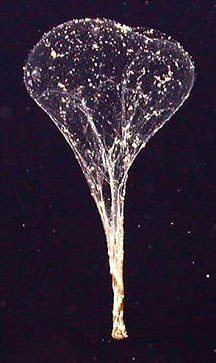 |
A giant larvacean and
its mucus net. Despite their
name, giant larvaceans are typically about 6 centimeters (about
2 1/2 inches) in length. The net is called a house, because the
larvacean lives in it, at the bottom. The nets can be over a
meter (yard) in diameter. When clogged (after about a day), the
nets are discarded, at which point they collapse and are called
sinkers. Sinkers carry great quantities of carbon to the seafloor.
Because they are large, they descend to the seafloor in a week
or so, much faster than most organic debris, which may take months.
It is estimated that about four such sinkers reach each square
meter (square yard) of the seafloor every day. Giant larvaceans typically live at depths from about 100 to 500 meters (yards). The net is lit by a light from the submersible craft which took its picture. (Monterey Bay Aquarium Research Institute, 2004; Robison, 2005) |
Sinkers apparently deliver a huge amount of carbon to the seafloor (Robison, 2005), much of which is consumed by the creatures that live on the seafloor and in its sediments (a portion of which is decomposed to the methane of the methane hydrates and the free gas below). The carbon that is converted to methane, as well as the carbon that is fully buried, are removed from the global carbon cycle, on both short and long time scales (several thousand to many millions of years). Consequently giant larvaceans have an extremely important role in maintaining the current level of atmospheric oxygen.
Giant larvaceans also depend upon oxygen. Giant larvaceans are chordates (animals with extended nerve bundles down their backs), just like us. Because they are animals (not specifically because they are chordates), they require oxygen. Where oxygen does not exist, neither do giant larvaceans. If giant larvaceans, or organisms that performed a similar ecological function (sending large packets of organic debris to the seafloor) existed during the last hundred million years of the Paleozoic (roughly 350 million to 250 million years ago), therefore, they could help explain the high levels of oxygen in that ancient atmosphere.
And, when the end-Permian ocean became anoxic, they would have died (though not all of them, obviously, because they are still around today). Their sinkers would have ceased dropping to the seafloor, and more unconsolidated fine organic particles would have become available for decomposition as they fell slowly through the water column. Had nothing else in the marine ecosystem been altered, this would have meant that more carbon rain would have been decomposed, and less would have reached the seafloor (ultimately resulting in a decrease of atmospheric oxygen).
Two additional factors, however, complicate this picture. On one hand, phytoplankton productivity would presumably have been declining as well, so less organic debris would have been produced in surface waters. Thus there would have been less carbon rain available for removal from the global carbon cycle. On the other, the anoxic condition of the deep ocean would have only allowed for anaerobic decomposition, a process much less efficient that decomposition by aerobes. Thus a greater proportion of the carbon rain that was produced would have made it to the ocean floor. The opposing effects of these various processes, together with unknown changes in the composition of the marine biota, make it impossible (at least with our current state of knowledge) to hazard guesses as to their impact on the level of atmospheric oxygen. But that they had the potential for major effects is clear.
Were giant larvaceans around during the
late Paleozoic and at the end of the Permian? We may never know
(although their major ecological importance may encourage paleontologists
to search for them). Giant larvaceans lack hard parts (as do their
nets), and organisms that lack hard parts rarely and only under
exceptional conditions fossilize. (The most common of such exceptional
conditions is anoxia and thus the same condition which may have
killed off any giant larvaceans then living would also have served
to help preserve their remains.) In addition, those seafloor sediments
in which they would have been preserved is, for the most part,
gone forever, as virtually all of the Permian seafloor has been
recycled by plate tectonics. Moreover, those small outcrops that
survived by becoming parts of continents (via the process called
obduction) may have been too altered by heat and pressure to possess
recognizable giant larvacean fossils.
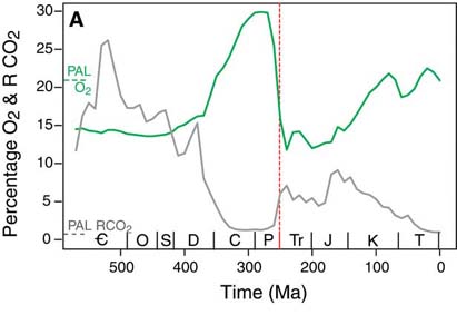
Whether it was due to the demise of oxygen producers, the oxygenic photosynthesizers (phytoplankton and terrestrial green plants), or due to demise of creatures like the giant larvaceans, which helped prevent atmospheric oxygen depletion, however, it is clear that something did happen at the end of the Permian which resulted in significant oxygen depletion. Atmospheric oxygen levels, which, due to the rise of the forests, had reached their highest ever (at about 30%, though it may have been as high as 35%: Berner, 2001) in the Early Permian, plummeted at its end (to perhaps 16%: Berner, 2002; Huey and Ward, 2005). The fall continued through the Early Triassic, reaching perhaps 12% at its lowest point, the lowest since trees and other green plants colonized the land. At the end of the Triassic, the situation may have shown no improvement, with oxygen levels remaining at close to 10% (Falkowski, 2005).
Organisms which had fully adapted to
the high levels of oxygen of the earlier Permian (roughly 286
million years ago and thereafter) would have been prime candidates
for extinction when oxygen levels fell. Creatures which previously
enjoyed high levels of oxygen at higher altitudes would have been
forced to descend to close to sea level to obtain similar quantities
of oxygen; those at sea level already would have had nowhere to
go because the high oxygen levels formerly found at that elevation
simply no longer existed (Huey and Ward, 2005). Oxygen deprivation,
therefore, is a likely major cause of the End-Permian extinction
of terrestrial animals.
CONTINUE TO NEXT SECTION (Early
Triassic Aftermath, Part 2)
RETURN
TO CONTENTS